Linear Correlation

Linear regression is commonly used to model the relationship between two variables, for example, the size of an apartment and its electrical energy consumption.

Another example is the current drawn in a magnetic winding and the supply voltage [1]. Here, the independent variable is the supply voltage \(x\), whereas the dependent variable is the current \(y\). Values of \(x\) and \(y\) measured in 10 tests are given in the table and scatter plot below.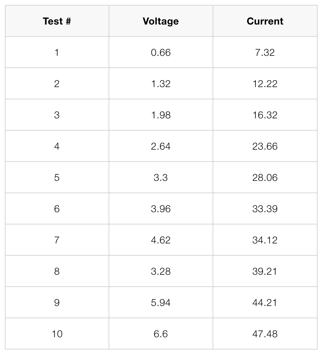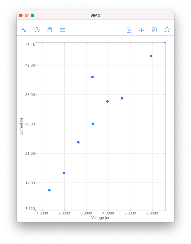

As we can see from the scatter plot above, the data \((x,y)\) tend to fall along a line with positive slope. This  might suggest that \(x\) and \(y\) are somewhat linearly correlated. However, we have to be careful when making such an assumption. The validity of the assumption is always doubtful, unless we have conducted analyses to establish the adequacy of the linear model. Analyses can be performed using the function corrcoef in SIMO or Console. This is explained in the following section.

Correlation Coefficient
Correlation coefficient is used to measure the linear relationship between two variables. For the variables \(x\) and \(y\), their correlation coefficient is defined as 
$$\rho_{xy}=\frac{\sigma_{xy}}{\sigma_y\sigma_x},$$
where \(\sigma_{xy}\) is the covariance, and \(\sigma_x\) and \(\sigma_y\) are the standard deviations of \(x\) and \(y
\), respectively. 

• The variables \(x\) and \(y\) are called correlate if \(\rho_{xy}\neq 0\).
• It always holds that \(-1\leq\rho_{xy}\leq 1\).
• Complete positive correlation means \(\rho_{xy}=1\), which suggests that \((x,y)\) fall along a line with positive slope.
• Complete negative correlation means \(\rho_{xy}=-1\), which suggests that \((x,y)\) fall along a line with negative slope. 

The function corrcoef can be used to compute the sample correlation coefficient \(r_{xy}\), which is an estimation of \(\rho_{xy}\). This is shown in the example below.

Input

Output

The value in R(1,2) gives the sample correlation coefficient \(r_{xy}\approx 0.9479\). Since \(x\) and \(y\) are real numbers, the matrix R is symmetrical. If \(x\) or \(y\) was complex, R(1,2) would be a complex conjugate of R(2,1). 

Hypothesis Testing
Now, we perform further analysis to confirm that \(x\) and \(y\) are indeed linearly correlated. We test the null hypothesis \(H_0:\rho_{xy}=0\) against \(H_1:\rho_{xy}\neq 0\). The null hypothesis \(H_0\) suggests that \(x\) and \(y\) are uncorrelated, whereas the alternative hypothesis \(H_1\) suggests that they are somewhat linearly correlated. 

The null hypothesis \(H_0\) can be rejected if the \(p\)-value is less than a given significant level \(\alpha\). A low \(p\)-value suggests that observing the null hypothesis \(H_0\) is unlikely. The \(p\)-value for \(\alpha=0.05\) is given by P(2,1), which is almost zero. This suggests that it is extremely unlikely that \(x\) and \(y\) are uncorrelated.

If \(\alpha\) is not specified in the input argument, the default value \(\alpha=0.05\) is used. To specify a custom \(\alpha\), say, 0.1, use corrcoef(x,y,'alpha',0.1).

Confidence Interval
Finally, we obtain the \((1-\alpha)\%\) confidence interval of \(\rho_{xy}\) with the default \(\alpha=0.05\). This is given by RL(2,1) and RU(2,1) in the above example. As a result, we conclude that
$$0.7895\leq\rho_{xy}\leq 0.9879.$$

😎 To know more about the topic and usage of corrcoef, check out the document pages in our apps. Thanks. 😎

References
[1] Douglas Montgomery and George Ringer, Applied Statistics and Probability for Engineers, 6th edition, Wiley, 2014.