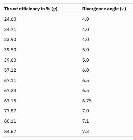
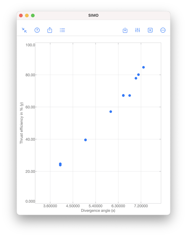
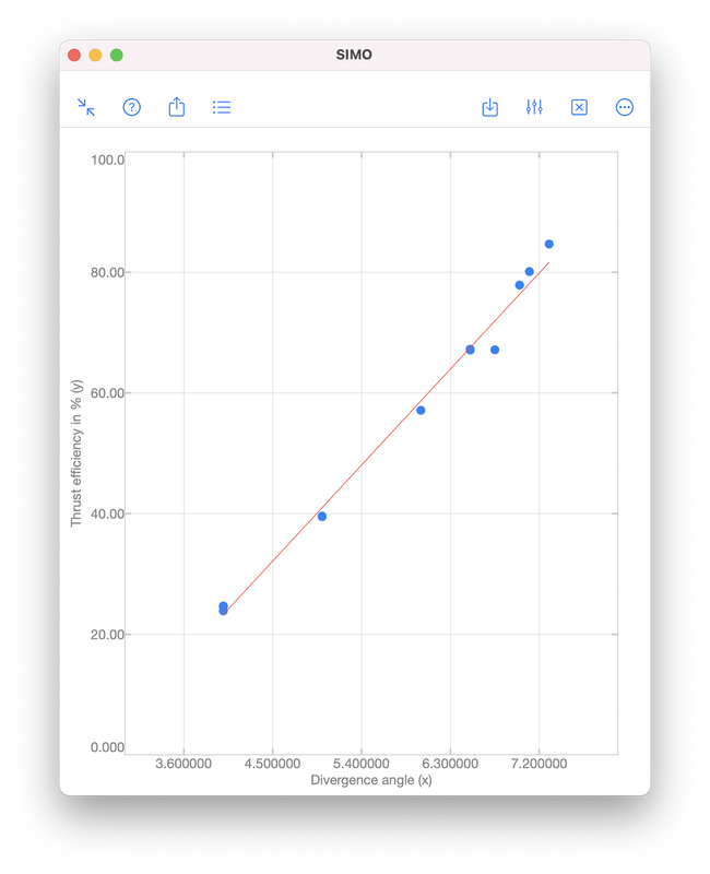
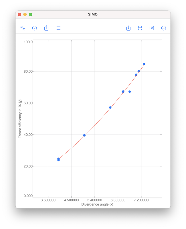
Polynomial Regression

12/24/2022

Polynomial regression is a technique to model the dependence of data collected in an experiment. The dependence is represented by a polynomial:
$$f(x)=a_0x^{n}+a_1x^{n-1}+\cdots+a_{n-1}x+a_n,$$
where $x$ is a real number. The integer $n\geq 0$ is called the order of the polynomial, which is defined as the highest power among the terms with non-zero coefficient. For examples,
$$-5,\quad x+1,\quad 2x^3+x^2+1$$
are zeroth ($n=0$), first ($n=1$) and third ($n=3$) order polynomials, respectively. Note that $0\cdot x^2+x+1$ is a first order polynomial since the first term has zero coefficient.

Illustrative Example

To illustrate the idea of polynomial regression, we consider data collected during an experiment to determine the change in thrust efficiency (in percent) as the divergence angle of a rocket nozzle changes (see [1], p. 530):

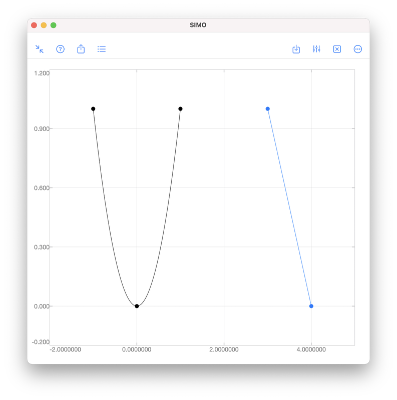
The divergence angle, denoted as $x$, is the independent variable. The thrust efficiency, denoted as $y$, is the dependent variable. First of all, we visualise the data by constructing a scatter plot using the script below.

Let $(x_i,y_i)$ be a given data point for $i=1,2,\ldots,N$. We want to find a polynomial $f$, such that $y_i\approx f(x_i)$ for all $i$.

Interpolation

Interpolation requires the polynomial passing through all given data points, i.e., $y_i=f(x_i)$ for all $i$. However, this often requires a high order polynomial because the order grows with the number of data points:

In general, a polynomial of order $N-1$ is required to interpolate $N$ points.

As shown in the following figure, a straight line, i.e., first order polynomial, is required to interpolate 2 points. To interpolate 3 points, a polynomial of at least order 2 is required (unless all 3 points fall on a straight line).

When the order is large, the polynomial exhibits oscillatory behaviour. This is known as the Runge's phenomenon, as seen from the figure blow.

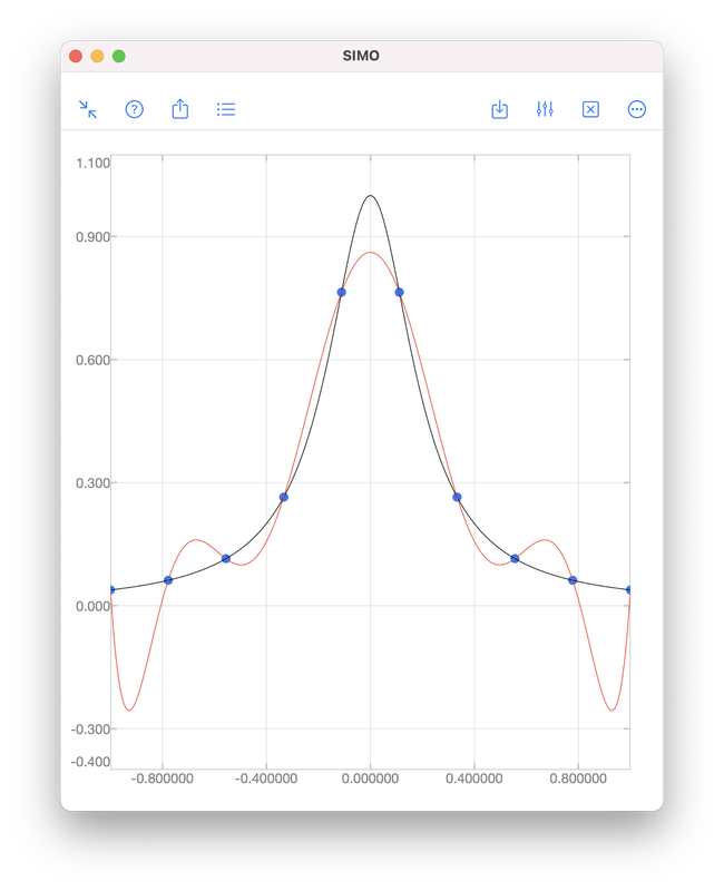
In this above figure, the blue dots represent samples of the black curve. There are in total 10 points and hence interpolation requires a 9th order polynomial, as shown by the red curve. We see that the red curve is oscillatory while the original curve (black) is not.

Regression

As we have seen, it is sometimes undesirable to force a polynomial to strictly pass through all data points. A better approach is to look for a polynomial that is "good enough". That means, we find a polynomial such that the error
$$e=\sqrt{\sum_{i=1}^N\left[y_i-f(x_i)\right]^2}$$
is minimised. Obviously, for interpolation, the error is zero. When interpolation is undesirable, we will accept a non-zero but minimised error $e$.

To perform polynomial regression:

Select a suitable polynomial order $n$. The order $n$ should be small, such as, 1, 2 or 3.
Find the coefficients $a_0,a_1,\ldots,a_n$ such that the error $e$ defined above is minimised.
Evaluate the fitness of the regression. If needed, choose a different $n$ and perform Step 2 again.

The coefficients $a_0,a_1,\ldots,a_n$ in Step 2 can be obtained by solving a least square problem using QR decomposition. A brief description can be found in the document page of polyfit included in SIMO or Console.

The coefficients can be obtained by SIMO or Console using the function polyfit, as shown below.

The output coefficients are 17.680815 and -47.420696. Therefore, the polynomial obtained is
$$f(x)=17.680815x-47.420696.$$
The error $e$ is given by S.normr, which is 6.9987482. As shown below, the error can be improved to 4.971942 by using a second order polynomial
$$f(x)=1.4670472x^2+1.3837119x-4.4594937.$$
For the meanings of s.R and s.df, please see the document page of polyfit included in the apps.

That is it for the post. If you have any question, feel free to leave comments. Thanks.

References

[1] Montgomery Runger Hubele, Engineering Statistics, 5th edition, Wiley, 2011.
[2] Gene H. Golub and Charles F. Van Loan, Matrix Computations, 4th edition, The Johns Hopkins University Press, 2013.

1 Comment